Let’s play a simple statistics game. I’m looking at a normal distribution with unit variance (which you can’t see) and I’m going to randomly sample a point from it, which I’ll share with you. You’ll then guess the mean of the distribution.
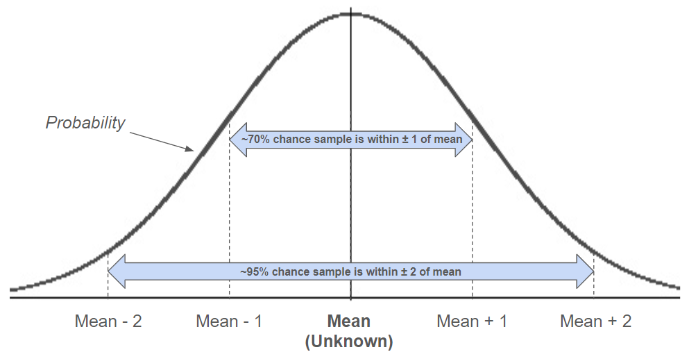
Let’s say the random sample has a value of 6. What would your guess be for the mean of the distribution it came from?
Given the limited amount of information available, guessing 6 seems like a logical choice. The true mean could, of course, be any number in theory, but a distribution centered at 6 would be most likely to have generated the observed value. Accordingly, this approach is known as the Maximum Likelihood Estimator (MLE), and it is in fact “best”, on average. You’re certainly free to take other approaches, like guessing 50% of the sample value, or always guessing 3 regardless of sample value, and while these approaches will do better for certain distribution means (ones that are smaller or near 3, respectively), for most they’ll perform worse.
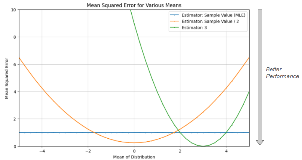
The Mean Squared Error (MSE) quantifies this performance, representing the expected square of the difference between a guess and the true mean for a particular estimation approach. Here, “expected” means that the evaluation considers all possible samples (and their corresponding probabilities) associated with a particular mean. When you guessed 6 as the mean of the distribution above, this single guess could have had any error (since the mean could be a number like 1,000, though this is exceedingly unlikely), and so that single comparison wouldn’t provide a meaningful view of estimator performance. Instead, we look at how the general approach (taking the mean to equal the observation) performs when repeated a large number (technically an infinite number) of times, and for the MLE see that we can expect an MSE of 1 for any distribution mean.
What is really meant by calling the MLE the “best” estimator is that no other approach can sit entirely beneath the blue line on the chart. As shown above, other estimators can do better for certain distribution means, but no approach can universally do better than the MLE.
We can also pose the same type of mean estimation problem in two dimensions. Let’s say I now have two normal distributions and will randomly sample a point from each, which I’ll share with you. You’ll then guess the mean of each distribution, with a goal of minimizing the total expected MSE across both.
Unsurprisingly, the MLE remains the best approach. Intuitively, it doesn’t seem possible to do better, regardless of the number of dimensions – the only information available is the sample, and the MLE represents the distribution most likely to have generated that sample. For an estimator to universally do better, it appears that additional information on the hidden distribution would be required, beyond the single sample.
However, in three dimensions we encounter something counterintuitive. Given a sample with the values x, y, and z, we can universally do better than the MLE by multiplying each value by a factor of (1 – 1/(x2+y2+z2)). For example, given x = 3, y = 5, and z = 1, we get a factor of (1 – 1/35), or ~97%, meaning we’d guess 2.91, 4.85, and 0.97 as the means of each dimension. As observed here, this factor “shrinks” each value toward 0, with a larger impact the closer the sample values are to 0.
This approach is known as the James-Stein estimator, and it’s applicable in three dimensions and above. Essentially, it allows for a “free guess” at the location of the distribution mean, which is made before seeing any samples (i.e., with no information) and then serves as the point toward which samples are “shrunk”. Generally, this guess is treated as the origin (as above), but this is mainly to simplify the math – the guess can be any point, and in the limit with an infinitely far off guess the James-Stein estimator generalizes to the MLE.
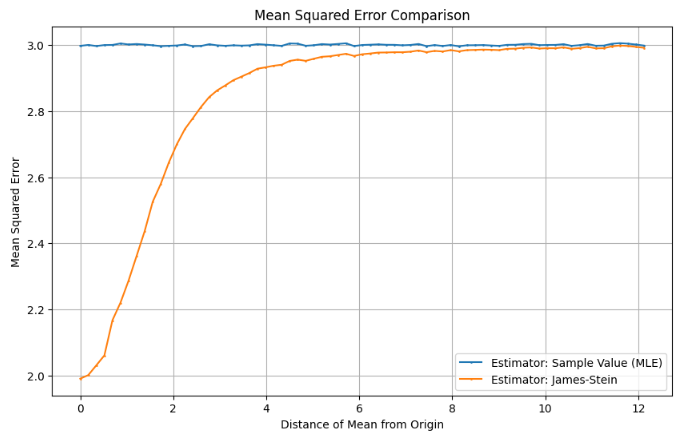
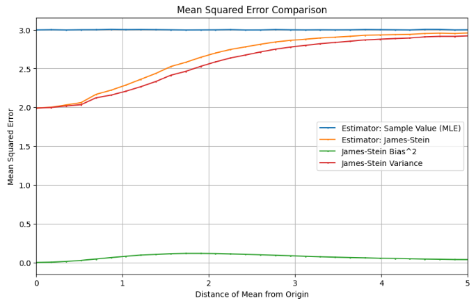
We can start to build some intuition around the James-Stein estimator based on the above chart showing its MSE vs. the MLE. It turns out that the improvements are highly concentrated in the region where the distribution mean is near the shrinkage point (the origin in this case), which makes sense as the operation pushes each guess in that direction (as seen above with the multiplier of 97%). Within this region it’s acting somewhat similar to the “Sample Value / 2” estimator, which also improved on the MLE for small distribution means by reducing the value of each estimate.
The more counterintuitive behavior occurs as the distribution mean moves further from the shrinkage point, where we’d expect the shrinking to negatively impact performance. Instead, the James-Stein estimator approaches the MLE as this distance increases, but always remains slightly more accurate. This behavior is driven by the structure of the shrinkage factor – it’s set up to shrink less as distance increases, allowing the estimator to remain below the MLE. For example, with a sample of [10, 10, 10], the scaling factor would be 99.7%, and it continues to drop exponentially as the distance from the shrinkage point increases.
When first learning about the James-Stein estimator, the above points made some sense to me, but my main question, which they didn’t answer, was why there was “room” to universally outperform the MLE. As we saw in one dimension, it seems like any attempt to beat it for some distribution means should result in worse performance on others. I still don’t have a truly satisfactory understanding of why this is the case, but below will attempt to shed a bit of light on what’s going on.
One concept central to understanding the James-Stein estimator is the fact that the MSE has two components, bias and variance (MSE = Bias2 + Variance). Bias represents the direction (if any) in which an estimator is off, on average, while variance represents the degree to which the estimates are spread out from each other. The MLE is an unbiased estimator because it’s equally off in all directions, on average, and so its MSE is driven solely by the variance in its estimates (which are directly driven by the spread of the underlying distribution). A modified MLE which adds 1 to each sample value would have a bias of 1 and the same variance, and the “always guess 3” estimator has zero variance with increasing bias as the distribution mean moves from 3. The James-Stein estimator works by reducing variance (pushing the estimates closer to each other) at the cost of bias (toward the shrinkage point) in a way that ensures the total MSE improves regardless of the distribution mean.
While the math works out, it’s still difficult to wrap one’s head around why the James-Stein estimator can leverage bias in such a way. This unintuitive nature stems from the way the bias and variance tradeoff changes with dimensionality.
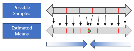
Put most simply, these differences are due to the fact that there’s a lot more space in higher dimensions, which reduces the impact of the James-Stein estimator to bias and increases its impact on variance. This difference can be seen in the comparison below between the James-Stein estimator impact in one dimension vs. two for an example mean close to the shrinkage point.
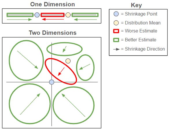
In one dimension, any samples which sit between the distribution mean and the shrinkage point will be further from the mean after shrinkage, while the rest of the samples will move closer. In two dimensions, these points where accuracy degrades are instead captured by an oval sitting between the shrinkage point and distribution mean, with the rest of the space seeing improvement. While not mathematical, it’s easy to see looking at the above that the green space represents a significantly larger portion of the total space in two dimensions than in one.
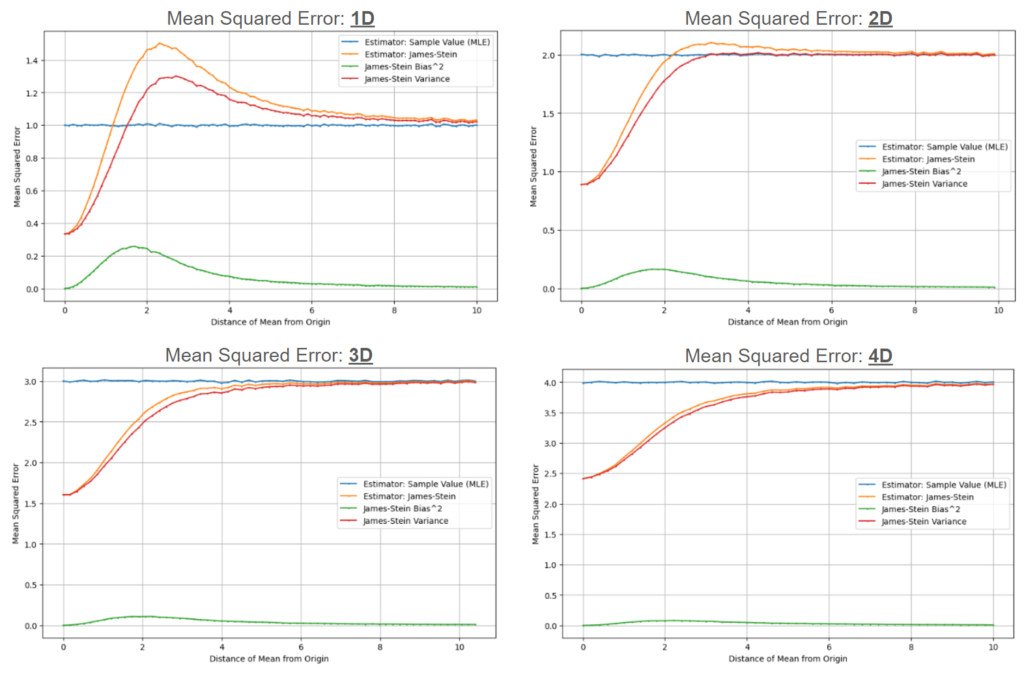
The same trend continues as we move to three dimensions and beyond, with the negatively impacted space growing smaller and smaller in relation to the total volume. We can see the impact this has on the bias and variance contributions as we move through the dimensions (note that the charts below show a modified James-Stein estimator with the shrinkage factor floored at 0 to simplify the behavior).
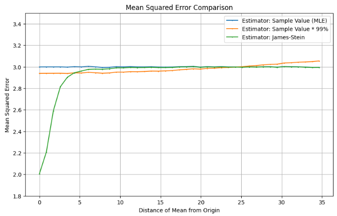
This change in the relationship between bias, variance, and the shrinkage factor creates an opening for improving on the MLE at higher dimensions. However, one fact I find comforting is that, for the exceedingly vast majority of distribution means, the James-Stein estimator is the MLE. As the problem is framed, the distribution mean can sit anywhere in the 3D (or 4D, etc.) space, and so in general any chosen shrinkage point will sit an (essentially) infinite distance away. Obviously this isn’t true for any estimation of this sort in practice – in these situations we generally have established bounds within which the distribution mean is likely to reside. However, the knowledge of these bounds provides additional information that allows us to specify an estimator that outperforms both the MLE and James-Stein estimators! For example, if we had information indicating the mean would be within 25 units of the origin, we could simply take the sample value * 99% as our estimator (which outperforms on average since the volume associated with means 5 to 25 units away from the origin is over 100x the volume of means 0 to 5 units away).
Overall, my main takeaway from the James-Stein estimator is that it can be difficult to wrap one’s head around the differences that emerge when dealing with increased dimensionality. I’m reminded of the fact that a random walk in 2D is guaranteed to hit any point an infinite number of times, while a random walk in 3D may never even return to where it started. Things are simply different in higher dimensions, often in unintuitive ways. At least in up to three dimensions we can ground ourselves in the real world – but I imagine many other surprises lurk further beyond.